Deep Learning for Natural Language Processing – Part I
Author – Wilder Rodrigues
Nowadays, the task of natural language processing has been made easy with the advancements in neural networks. In the past 30 years, after the last AI Winter, amongst the many papers have been published, some have been in the area of NLP, focusing on a distributed word to vector representations.
The papers in question are listed below (including the famous back-propagation paper that brought life to Neural Networks as we know them):
- Learning representations by back-propagating errors.
- David E. Rumelhart, Geoffrey E. Hinton & Ronald J. Williams, 1986.
- A Neural Probabilistic Language Model
- Yoshua Bengio, Réjean Ducharme, Pascal Vincent, Christian Jauvin, 2003.
- A Unified Architecture for Natural Language Processing: Deep Neural Networks with Multitask Learning
- Ronan Collobert, Jason Weston, 2008.
- Efficient Estimation of Word Representations in Vector Space.
- Tomas Mikolov, Kai Chen, Greg Corrado, Jeffrey Dean. 2013
- GloVe: Global Vectors for Word Representation.
- Jeffrey Pennington, Richard Socher, Christopher D. Manning, 2014.
The first paper on the list, by Hinton et al, was of extreme importance for the development of Neural Networks, it made all possible. The other papers targeted NLP, bringing improvements to the area and creating a gap between Traditional Machine Learning and Deep Learning methods.
If we look at the Traditional Machine Learning approaches compared to what is done now with Deep Learning, we can see that most of the work done is related to modelling the problems other than engineering features.
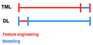
In order to understand how the Traditional Machine Learning approach has more feature engineering than its Deep learning counterpart, let’s look at the table below:
|
Representations of Language |
||
| Element | TML | DL |
| Phonology | All phonemes | Vector |
| Morphology | All morphemes | Vector |
| Words | One-hot encoding | Vector |
| Syntax | Phrase rules | Vector |
| Semantics | Lambda calculus | Vector |
The words in a corpus are distributed in a vector space, where the Euclidean distance between words will be used to measure their similarities. This approach helps to identify gender and geo location given a word within a context. The image below depicts the Vector Representations of Words:
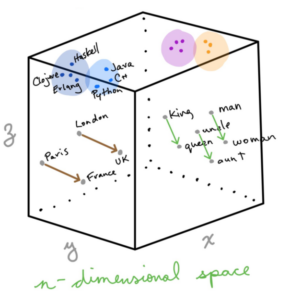
Source: Jon Krohn @untapt – Safari Live Lessons
Those associations are done automatically thanks to Unsupervised Learning, a technique that dispenses the need for labeled data. All a Word to Vector approach needs is a corpus of natural language and it will learn it by clustering the words.
When it comes to Traditional Machine Learning methods, instead of a vector representation, we have one-hot encoding. This technique works and has been used for a long time. However, it is infinitely inferior to vector representations. The image below depicts how One-hot encoding works:
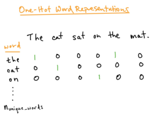
Source: Jon Krohn @untapt – Safari Live Lessons
And in the table below we summarise how both methods can be compared:
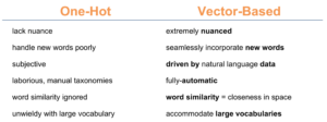
Source: Jon Krohn @untapt – Safari Live Lessons
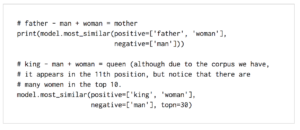
Another important add-on from Vector Representations of Words is word-vector arithmetic. One can simply deduct and add words from/to a given word to get its counterpart. For instance, let’s say that we do the following:
- King – man + woman = Queen.
We will demonstrate how it’s done with some code further in the article.
Although not in a very detailed way, here are some other important terms and architecture details that we have to touch. For instance, how does the algorithms get to understand words from a given context in a corpus or vice-versa?
To start with, let’s look at some terms:
- Target word:
- The word to be predicted from a source of context words.
- Context words:
- The words surrounding a target word.
- Padding:
- The number of characters to the left of the first context word and to the right of the last context word.
The image below depicts how the algorithms work in with target and context words:
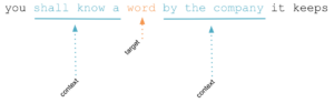
John Rupert Firth, 1957
Source: Jon Krohn @untapt – Safari Live Lessons
The word2vec implementation of 2013 paper by Mikolov et al comes in two flavours: Skip-Gram; and Continuous Bag-of-Words (i.e. CBOW).
- Skip-Gram:
- It predicts the context words from the target words.
- Its Cost Function maximises the log probability of any possible context word given the target word.
- CBOW:
- It predicts the target word from the bag of all context words.
- It maximises the log probability of any possible target word given the context words.
- The target word is the average of the context words considered jointly.
- Why continuous? Because Word2Vec goes over all the words in the corpus continuously creating bags of words. The order is irrelevant because it looks at semantics.
As it has been shown above, the implementations do exactly the inverse of each other. Although it might be seen as an arbitrary choice, statistically speaking, it has the effect that CBOW smoothes over a lot of the distributional information (by treating an entire context as one observation), whilst its counterpart, Skip-Gram, treats each context-target pair as a new observation, and this tends to do better when we have larger datasets.
HOW TO GET IT WORKING?
Now that we have seen some theory about NLP and Vector Representations of Words, let’s deep dive into some implementations using Keras, word2vec (the implementation of the 2013 paper), Deep (using fully connected networks) and Convolutional Networks.
As an example, we will the MNIST dataset. It might look exhausting, since everybody does it, but having a well-curated dataset is important to start on the right foot. Our first example will just demonstrate the use of word2vec.
Import Dependencies
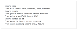
What to keep in mind for further research?
- NLTK
- Pandas
- ScikitLearn
- Gensim
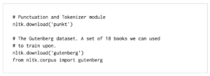
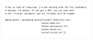
Load Model and Data
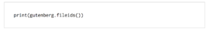
If you want to have a look at the books available in the Gutenberg dataset, please execute the line below:
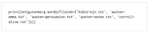
Load Sentences
If you want to know how many words are in the set we loaded, please execute the line below:
Run the Word2Vec Model
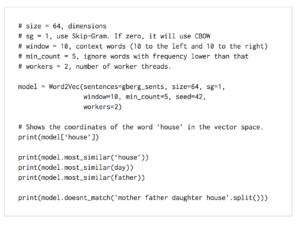
Similarities
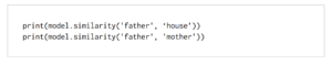
Arithmetics
REDUCE WORD VECTOR DIMENSIONALITY WITH T-SNE
t-Distributed Stochastic Neighbour Embedding (t-SNE) is a technique for dimensionality reduction that is particularly well suited for the visualisation of high-dimensional datasets.
Although our vector space representation doesn’t have many dimensions, we got only 64, it is still enough to get humans confused if we try to plot the 8667 words from our vocabulary in a graph. Now imagine how it would work with 10 million words and thousand dimensions! Our friend that was shortly explained above can help us with that. Let’s get to the code and plotting.
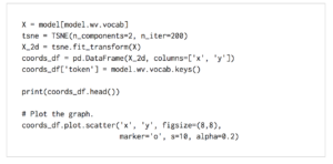
Applying t-SNE
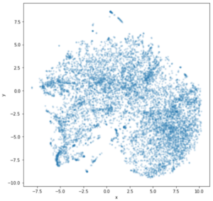
Doesn’t help to see it like this. Let’s try something else instead:
BokehJS
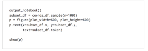
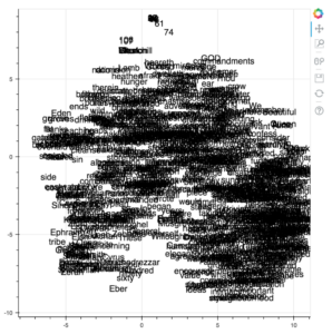
You can use the Bokeh controls to zoom in and move around the graph.
Acknowledgements
Thanks for taking the time to read this article and do not hesitate to give your feedback.
The source code is available via Github: https://github.com/ekholabs/DLinK
Interested in applying Machine Learning at your company? See how experts at Trifork can help you. More info here.
Author – Wilder Rodrigues