Deep Learning for Natural Language Processing – Part II
Author – Wilder Rodrigues
Wilder continues his series about NLP. This time he would like to bring you to the Deep Learning realm, exploring Deep Neural Networks for sentiment analysis.
If you are already familiar with those types of network and know why certain choices are made, you can skip the first section and go straight to the next one.
I promise the decisions I made in terms of train / validation / test split won’t disappoint you. As a matter of fact, training the same models with different sets got me a better result than those achieved by Dr. Jon Krohn, from untapt, in his Live Lessons.
From what I have seen in the last 2 years, I think we all have already been through a lot of explanations about shallow, intermediate and deep neural networks. So, to save us some time, I will avoid revisiting them here. We will dive straight into all the arsenal we will be using throughout this story. However, we won’t just follow a list of things, but instead, we will understand why those things are being used.
What do we have at our disposal?
There is a famous image that does not appear only on several blog posts about Machine Learning, but also on Meetup meetings, conferences and company-closed presentations. Although I wouldn’t add it here just for the sake of it, I think it’s interesting to get the audience to see some ofthe network architectures we currently have.
The people behind the @asimovinstitute came up with a quite interesting compilation. See for yourself:
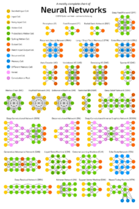
The Neural Network Zoo, by the Asimov Institute — https://www.asimovinstitute.org/
There are many more curiosities and things to learn about the Neural Network Zoo. If that’s something that would make you more interested in Neural Networks and their intrinsic details, you can find it all in their own blog post here: https://www.asimovinstitute.org/neural-network-zoo/.
For this story, we are going to focus on a Feedforward Neural Network. If you paid attention to the image above, it won’t be difficult to spot it. Otherwise, please refer to the image below:
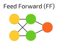
That is a pretty simple network! But no worries, we will be stretching it a bit, making it deeper. However, before we do that, let’s try to get a couple of things clear:
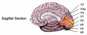
- Do you know about the Primary Visual Cortex? Since I can not hear your answer, I will just assume you don’t. So, there goes a fun fact: the Primary Visual Cortex is also known as V1. It’s called V1 because that’s like a first layer; it recognises the shapes of what we see. As the complexity of the information flowing increases, the layers dealing with it get more specialised and they have higher numbers associated with them. The picture below gives an idea about what I mean:
- You might have seen network architectures starting from bottom to top, or top to bottom, or sideways; even if those drawings were modeling the same type of network. This behavior doesn’t seem to be very consistent, and in addition to that, most of the papers or articles I have read depict neural networks starting either from bottom to top or left to right. If I have to draw a network architecture here, I will stick with the left to right style.
Now moving on to some more technical aspects of our Feedforward Neural Network, it’s time to actually define it. To get to work with word embedding vectors, as we did in the first part of this series, we have to define a very specific layer in our architecture. Along with this mysterious layer, we will also use a couple of other layers that are needed to achieve our goal.
In the list below, I pinpoint the types of layers we will be using for now:
- Embedding Layer: this layer is used to create a vector representation of the words in our document.
- Flatten Layer: after we have our vector, we flat it out in order to apply dimensionality reduction and get a 1D vector.
- Dense, or Fully Connected, Layer: a layer which has its neurons connected to all the other neurons in the previous layer.
Okay, we got the layers, but now what? There are other things to consider, like regularisation; cost function; activation function; and train/validation/test split. How are we going to deal with those details? Before we get to the code, let’s follow a few baby-steps through the sections below.
Regularisation
The goal of regularisation is to reduce overfitting. Although I really feel excited with the idea to talk about Weight Decay, Dropout and drawing formulas here, I won’t get into those details because if you want to learn about Deep Learning for NLP, I expect you to know about regularisation.
For the sake of it, we will be using Dropout. If you don’t know that much about it, please refer to Professor Geoffrey Hinton’s paper, published in 2013: https://www.cs.toronto.edu/~hinton/absps/JMLRdropout.pdf.
Cost Function
Okay, we got some details about the layers and the regularisation technique we will be using, now let’s try to get some intuition about the Cost Function we chose, why we did it and what else we had at our reach:
- Mean Squared Error: it is defined as 1/m * sum(Yhat, Y) ** 2, where the Yhat is defined by the hypotheses function (e.g. 𝜃0 + 𝜃1*x, etc.). The MSE is mostly used with Linear Regression because its hypotheses is linear and hence it generates a bowl, or convex, shaped function. By being convex-shaped, it helps to achieve global optimum during Gradient Descent. But wait, we will be working on a Classification problem and our hypotheses function will be non-linear (will talk about it later). It means MSE is not my choice for this problem.
- Cross Entropy: using Cross Entropy with Classification problem is the way to go. It differs from the MSE due to its nature and the shape its function has. Its equation is given by -1/m * sum(Y * log(Yhat) + (1 – Y) * log(1 – Yhat)). Just like with MSE, here we want the loss to be as small as possible. Let’s assume that Y equals to 1. By doing so, the second term of the equation, (1 – Y) * log(1 – Yhat), equals to 0, therefore canceled. In the remaining term, we have Y * log(Yhat), here we want Yhat to be as big as possible. Since it is calculated by the Sigmoid function, it cannot be bigger than 1. Now if we look at the other side of the spectrum, and have Y equals 0, then the first term is canceled and in that case we want Yhat to be small. I think you get the rest.
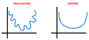
Non-Convex vs. Convex Functions. Pretty hard to find a global optimum in the former.
Gradient Descent Optimisation
We have already been through a lot without writing one single line of code. Please, bare with me here.
The goal of the Gradient Descent is to find a global optimum, that’s why the non-convex function is bad for such a task. The way it works, along with the minimised loss, is that for every training iteration it takes a small step towards the global optimum. Those steps are calculated based on the weights minus the learning rate times the derivative of the weights. The latter gives the changes in the weights per iteration. To put it in a more mathematical way, that’s how we update the weights during the gradient descent steps: w = w – ⍺ * dJ(w,b)/dw. That’s the most simple version of it, but there are some others that makes learning incredible faster compared to this one. One last thing: you might have noticed the ⍺, or learning rate. That’s a hyper-parameter that we use to tune the learning. When it’s too big, the steps might make the gradient descent hard to converge, and just keep moving from one side of this bowl to the other; if the number is too small, then it will take longer to learn.
For our exercise, we will be using Adam. This optimiser was first published in 2015, by Diederik P. Kingma and Jimmy Li Ba, from the University of Amsterdam and the University of Toronto, respectively. Adam combines momentum and RMSProp, which are both optimisation algorithms. Due to this combinations, Adam has been recognised as the best option when it comes to Deep Learning problems. In the “CS231n: Convolutional Neural Networks for Visual Recognition” developed by Andrej Karpathy, et al., at Stanford University, it is also suggested as the default optimisation method.
The implementation of Adam, which uses exponentially weighted average, to achieve momentum, and root mean square (RMS, from the RMSProp), is quite interesting and lengthy. I will share an image of a handwritten version of it, just to give you an idea about how the weights are updated using Adam.
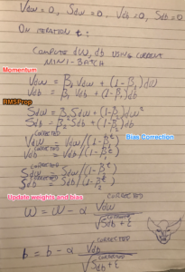
Adam: Adaptive Moment Estimation.
Activation Function
I almost forgot about that! We are going to use 2 different activation functions to work on this sentiment analysis problem. In the hidden layer, we will use the Rectified Linear Unit (ReLU) and as the output activation, we will use the Sigmoid function.
Perhaps it enough to show the graphs of both functions here. If you need some more details, I will add some references at the bottom of the paper so you can go straight to the source.
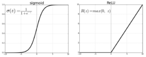
Sigmoid and ReLU activation functions.
Just a few details on the decisions made, we are using sigmoid for our hypotheses because we have a binary classification, or univariate, problem. The output should be 1, if the review is positive, or 0 otherwise. If we would be dealing with a multivariate problem, or trying to estimate the likelihood of a given image be one of those represented in out N-classes problem, for example with the MNIST or CIFAR datasets, we would use a Softmax as it outputs a probability distribution over the output vector (our N classes).
Getting our Hands Dirty
That was a lot of information! But after deciding for our network architecture, regularisation, cost function and optimisation, now it’s time to actually get something done and see for ourselves what this can do. I will basically add some blocks of code, along with comments to explain why certain things are done the way they are, or at least the way I chose to do.
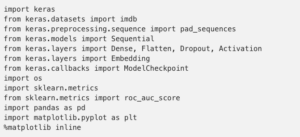
Import Dependencies
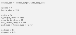
Set Hyper-Parameters
Load Data
![]()
Okay, now we defined some hyper-parameters and also loaded the data we will be training with. However, it would be interesting to understand why those things were done before we move on. Let’s take some time to explore those decisions now:
- Our Embedding space will have 64 dimensions;
- We are keeping a bag of 5000 unique words only.
- Top most frequent words to ignore;
- We are only looking at reviews that are 100 words max long.
After running the commands above, try to loop through some samples to see the length of the reviews before applying the preprocess step:
![]()
It should print something like the block below:

You will see the difference when we pre-process the data.
Restore Words from Index
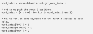
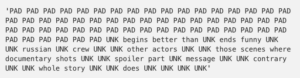
But why should we care about creating those indexes? Words with the indexes 0, 1 and 2 will be represented as PAD, START and UNK (i.e. unknown). Remember that we are not loading the full reviews, but only 5000 unique words per review and limiting a review length to 100. It will all make more sense once we pre-process the data. For now, let’s have a look at what we have as content for the first review:

The outcome should be something like the block below:
And if you want to compare it with the full review, try the following:

And the output should be:

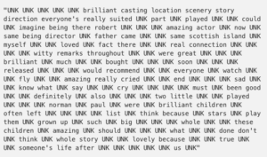
Preprocess Data
Now that we have pre-processed the data, let’s have a look at what happened to the reviews. Just as a remark, during pre-processing we have informed the max review length and also padding and truncating options.
Let’s start with the length of our reviews:
![]()
Now they are all 100 words long.
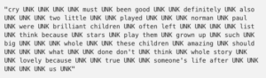
So, the pre-processing step already did something for us. Let’s have a look at what else changed by indexing the words of the first review:
![]()
And the output should be something like the block below:
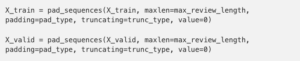
And what about the 6th review? Remember it had only 43 words? Let’s have a look:
![]()
And the output should be something like the block below:
It’s pretty clear what happened, right?
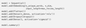
Design the Network Architecture
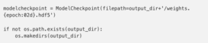
Create a Model Checkpoint
For every epoch we run, we want to save its weights. By doing so, we can later look at the epoch with the best accuracy on the validation set and then use it perform predictions on top of unseen data.
Compile and Run the Model
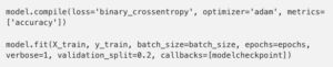
As you can see in the fit call above, I’m not using the the validation data provided in the IMBd dataset, but instead I’m just randomly splitting the train data, taking 20% of it to use for validation. I decided to do this, so after the model is trained I can run tests on top of the real validation data (as a test set) since it has not been seen by the model.
Run Prediction
![]()
Calculate the Average Under the Receiver Operating Characteristic (ROC) Curve (AUC)
![]()
Just a bit of information about the AUC: it gives you a better measurement method as it takes into account the True Positive Rate (TPR) and the False Positive Rate (FPR). To get those rates calculated, it does the following:
![]()
But for that to work, we also need to calculate the True Positive/Negative and False Positive/Negative values. To get that done, the AUC uses thresholds based on the predictions that were made, then calculating the TP/TN/FP/FN per threshold. The amount of TPF FPR points will be given by the amount of thresholds that were used. What would that be? All the unique predictions in the output. To understand it better, let’s have a look at the table below:
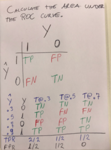
Use the TPR and FPR points that were calculated based on the 3 thresholds (i.e. T@.3, T@.5 and T@.7) plot a graph. The accuracy is then measured by the AUC.
After all that has been explained, feel free to execute the code below and plot your ROC graph:
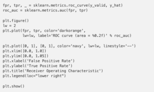
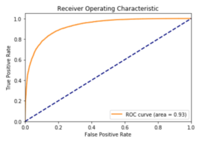
You should see something like the image below:
If you want to know if it worked okay, just play around with the output (i.e. y_hat). It contains all the predictions. The y_valid has the expected outputs. So, check both of them to see how far the predictions are. The code below can help you out a bit:
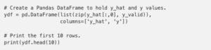
The output should be something similar to the table below:
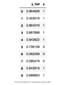
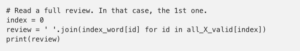
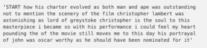
This review looks pretty positive:
Acknowledgements
Thanks again for following this far deep into the theory and code. I really appreciate those who take the time to read it.
The source code can be found here: https://github.com/ekholabs/DLinK
Interested in applying Machine Learning at your company? See how experts at Trifork can help you. More info here.