Smart energy consumption insights with Elasticsearch and Machine Learning

At home we have a Youless device which can be used to measure energy consumption. You have to mount it to your energy meter so it can monitor energy consumption. The device then provides energy consumption data via a RESTful api. We can use this api to index energy consumption data into Elasticsearch every minute and then gather energy consumption insights by using Kibana and X-Pack Machine Learning.

The goal of this blog is to give a practical guide how to set up and understand X-Pack Machine Learning, so you can use it in your own projects! After completing this guide, you will have the following up and running:

• A Complete data pre-processing and ingestion pipeline, based on:
  • Elasticsearch 5.4.0 with ingest node;
  • Httpbeat 3.0.0.
• An energy consumption dashboard with visualizations, based on:
  • Kibana 5.4.0.
• Smart energy consumption insights with anomaly detection, based on:
  • Elasticsearch X-Pack Machine Learning.

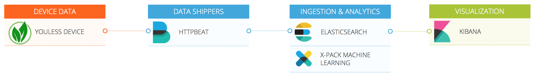
The following diagram gives an architectural overview of how all components are related to each other:

Installation

Prerequisites

The installation process of this guide is based on the use of Docker, so first make sure that you have the following tools installed:

• Docker Community Edition, v1.13.0, installation guide;
• docker-compose, v1.13.0, installation guide.

Git repository

All required files are available in the following GitHub repository: https://github.com/TriforkEindhoven/youless-elastic-ml

First clone the repository by executing the command:

git clone https://github.com/TriforkEindhoven/youless-elastic-ml.git

You will now have a directory youless-elastic-ml with the following content:

youless-elastic-ml
+-- containers
| +-- elasticsearch
| |  +-- config
| |  |   +-- elasticsearch.yml
| |  +-- Dockerfile
| +-- httpbeat
| |  +-- config
| |  |   +-- httpbeat.template.json
| |  |   +-- httpbeat.template-es2x.json
| |  |   +-- httpbeat.yml
| |  +-- Dockerfile
| +-- docker-compose.yml
+-- dashboards
|   +-- energyconsumption-dashboard.json
+-- scripts   
+-- create_pipeline.sh

To summarize, the repository contains the following content:

• An Elasticsearch directory for building our own Elasticsearch Docker image;
• A httpbeat directory for building our own httpbeat Docker image;
• A docker-compose configuration file which ties all Docker containers together;
• A json file which contains all Kibana visualization and dashboard definitions;
• A small script to register a pipeline into Elasticsearch.

Initial configuration

Before we can fire things up, we have to tell httpbeat what the url to the Youless device is. Open the file youless-elastic-ml/containers/httpbeat/config/httpbeat.yml in your favorite editor. The file starts with this fragment:

#================================ Httpbeat =====================================

httpbeat:

  urls:   
    -     
      cron: "@every 1m"     
      url: http://192.168.1.1/a?f=j     
      method: get     
      document_type: usage     
      output_format: json

Update the url property so that it points to the location of your Youless device. Make sure that the url ends with /a/f=j, as this is the end-point that httpbeat will be monitoring.

Fire it up – phase 1

Go to the youless-elastic-ml/containers directory and execute the command:
docker-compose up elasticsearch kibana

The command will start the elasticsearch and kibana containers. If everything went well, you can access the following end-points:

• Elasticsearch: http://localhost:9200
• Kibana: http://localhost:5601

Because in the Docker images Elasticsearch X-Pack security is enabled by default, you have to provide credentials when accessing the end-points mentioned above. The default credentials are:

• Username: elastic
• Password: changeme

For testing purposes, you can temporary disable X-Pack security by adding the following line to the file youless-elastic-ml/containers/elasticsearch/config/elasticsearch.yml and restart the Elasticsearch Docker container:

xpack.security.enabled: false

Pre-processing pipeline

At this point, if we would start httpbeat, it would post documents with the following structure to Elasticsearch:

{ 
  "@timestamp": "2017-05-07T01:11:21.001Z", 
  "beat": {
    "hostname": "1418d358bf51",
    "name": "1418d358bf51",
    "version": "3.0.0"
  },
  "request": {
    "method": "get",
    "url": "http://192.168.1.15/a?f=j"
  },
  "response": {
    "headers": {
      "Content-Type": "application/json"
    },
    "jsonBody": {
      "cnt": "38846,911",
      "con": "*",
      "det": "",
      "dev": "",
      "lvl": 0,
      "pwr": 186,
      "raw": 0,
      "sts": ""
    },
    "statusCode": 200
  },
  "type": "usage"
}

Although it’s nice to actually see some data, the document is a bit verbose and contains information that isn’t very useful. As you can see, the response.jsonBody object contains the actual information we are interested in.

In Elasticsearch 5.0 a new functionality called ‘ingest node’ with ‘pre-processing pipelines’ was introduced. We can use this functionality to pre-process the document before the actual indexing takes place. We will use the following pipeline definition:

{
  "description" : "Youless httpbeat events cleanup",
  "processors" : [
     { "rename": {
          "field": "response.jsonBody.pwr",
          "target_field": "power"
       }
     },
     {
       "rename": {
          "field": "response.jsonBody.cnt",
          "target_field": "total"
       }
     },
     {
       "rename": {
         "field": "response.jsonBody.lvl",
         "target_field": "level"
       }
     },
     {
       "gsub": {
         "field": "total",
         "pattern": ",",
         "replacement": "."
       }
     },
     {
       "remove": {
         "field": "request"  
       }
     },
     {
       "remove": {
         "field": "response"
       }
     }
  ]
}

The pipeline consists of the following six processing steps:

1. Rename the `response.jsonBody.pwr` field to the target field `power`;
2. Rename the `response.jsonBody.cnt` field to the target field `total`;
3. Rename the `response.jsonBody.lvl` field to the target field `level`;
4. In the `total` field, replace any `,` characters with a `.` character, so that it can be indexed as numeric field;
5. Remove the `request` field;
6. Remove the `response` field, because we moved all interesting fields to the root of the document.

Pre-processing the example document mentiond above, would result in the folowing document:

{
  "_index": "httpbeat-2017.05.07",
  "_type": "usage",
  "_id": "AVvgdgAsypvH30Ab6_DG",
  "_score": 1,
  "_source": {
    "@timestamp": "2017-05-07T01:11:21.001Z",
    "beat": {
      "hostname": "1418d358bf51",
      "name": "1418d358bf51",
      "version": "3.0.0"
    },
    "power": 186,
    "total": "38846.911",
    "level": 0,
    "type": "usage"
  }
}

For debugging purposes, we keep the beat field in the document. If you are not interested in this field, add the following processing step to the pipeline:

{
  "remove": {
    "field": "beat"
  }
}

Register the pipeline with Elasticsearch by executing the script:

youless-elastic-ml/scripts/create_pipeline.sh

Fire it up – phase 2

We are now ready to start the httpbeat container. Go to the youless-elastic-ml/containers directory and execute the command:

docker-compose up httpbeat

After one minute httpbeat should post its first data to Elasticsearch. You can check that documents are being indexed by executed the command:

curl localhost:9200/httpbeat-*/_count

The response should look like this:

{"count":1,"_shards":{"total":5,"successful":5,"failed":0}}

If everything looks alright, we are done with our data collecting setup. Hooray!

Kibana dashboards

Index pattern

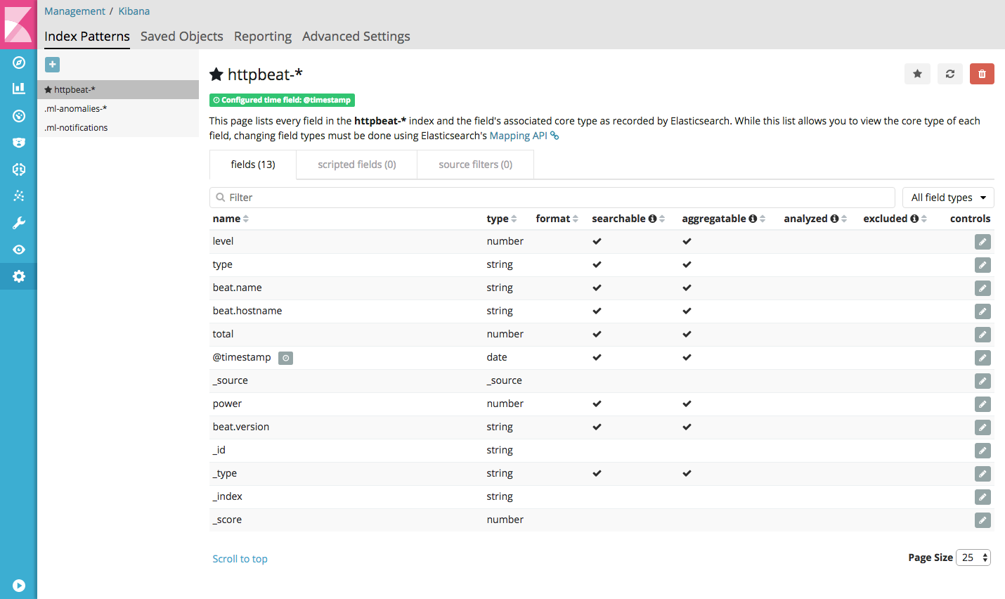
Before we can do anything in Kibana, we first have to create an index pattern. Let’s create an index pattern with the following settings:

• Index name or pattern: httpbeat-*
• Index contains time-based events: checked
• Time-field name: @timestamp

If the index pattern is created successfully, it should look like this:

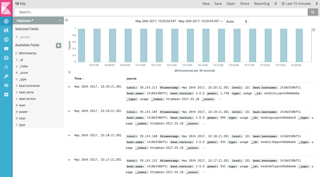
Go to the discover section of Kibana to see the indexed documents. You may have to update the time range (e.g. ‘Last 15 minutes’) to discover documents. If everything went well, you will see something like this:

Import visualization and dashboard definitions

At this point, you can start creating your own visualizations and dashboards. But to get you quickly up and running, we have prepared a energy consumption dashboard with a number of visualizations. To import these definitions, use the following steps:

1. In Kibana go to: Management / Saved Objects;

2. Click on the Import button, and upload the file: youless-elastic-ml/dashboards/energyconsumption-dashboard.json;

3. Check if the following objects have been imported correctly:

• Dashboards:
  • Energy consumption.
• Visualizations:
  • Average energy consumption;
  • Average daily consumption;
  • Average weekly consumption;
  • Average monthly consumption;
  • Min-median-max energy consumption;
  • Number of measurements;
  • Total energy consumption.

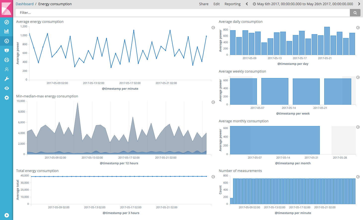
You can now open and see the Energy consumption dashboard with the different visualizations:

Machine learning

Kibana visualizations give a great overview of certain metrics within a time window. However, it can be hard to use them to spot anomalies, because they can easily get flattened in an aggregation. Furthermore, one can only analyze a limited number of visualizations at once. In a system with a lot of metrics, this scales very badly.

The machine learning product in Elasticsearch X-Pack uses the concept of jobs as the basis for data analysis. A job contains the configuration information to perform an analytics task. In this guide we will create a job that detects anomalies in the arithmetic mean of the value of power: mean_power.

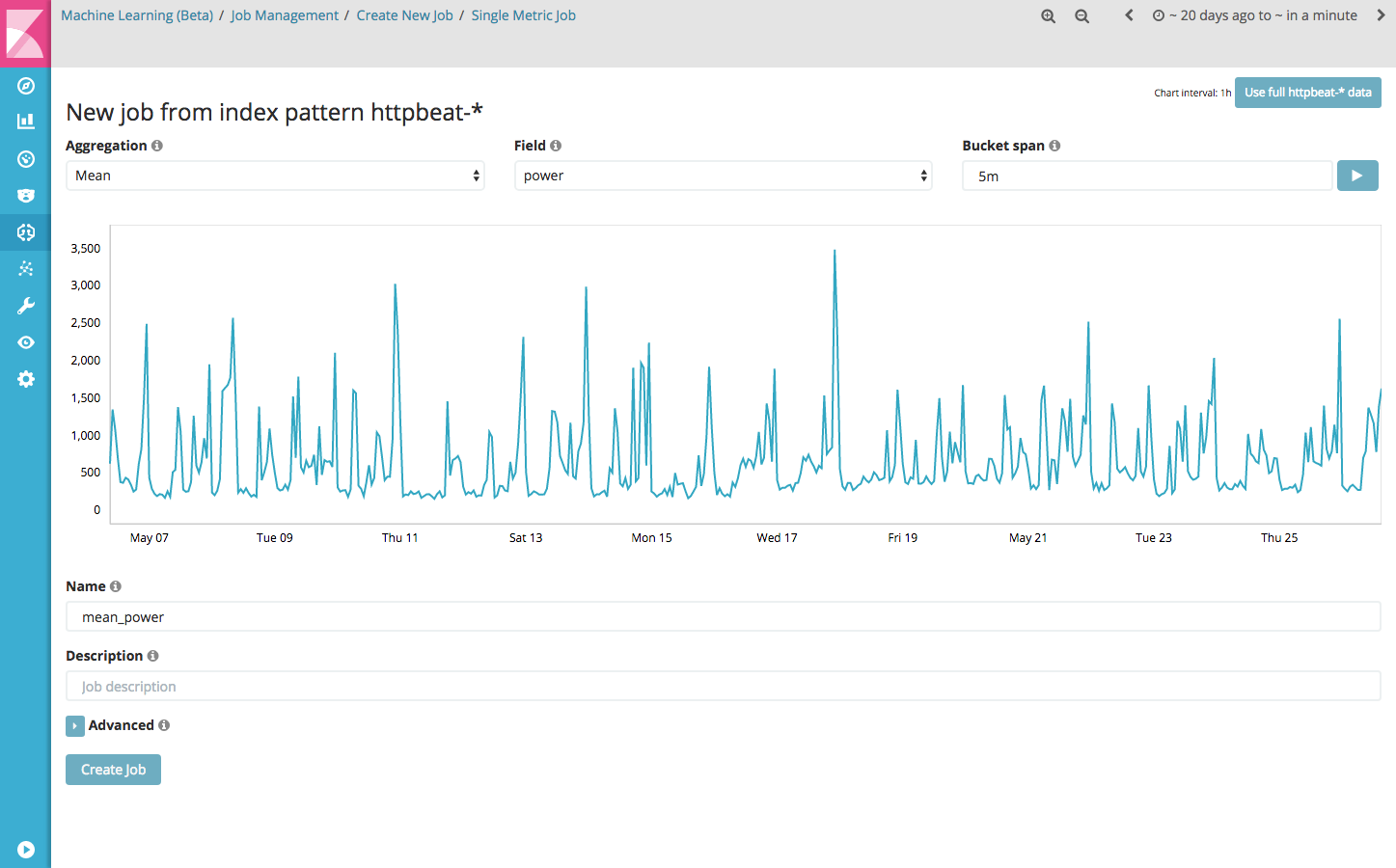
To create the mean_power job, use the following steps:

1. Create new single metric job;
2. Select the httpbeat-* index pattern;
3. Select the mean aggregation, with the field ‘power’ and a bucket span of 5m;
4. Click the ‘Use full httpbeat-* data’ button to load historical data;
5. Enter the name ‘mean_power’ as a job id;
6. Click the ‘Create job’ button.

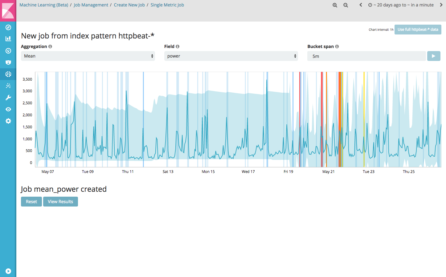
When you click the ‘Create job’ button, the full http-beat* data is fed into the model and the analysis begins. During the process it is interesting to see that it takes a while for the model to detect patterns in the data. Depending on the data, it may be the case that a number of anomalies already have been detected. After running the job creation process, the graph looks like this:

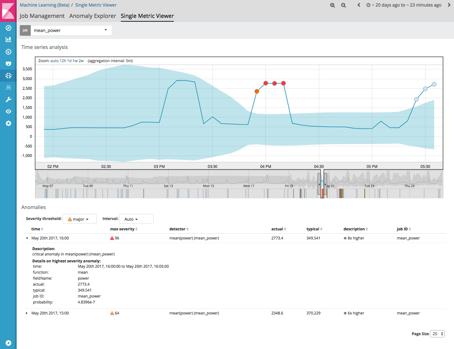
If you click the ‘View Results’ button, the Single Metric Viewer opens, which displays detected anomalies within a selected time window. For each anomaly, detailed information, like the actual value and the expected typical value are given.

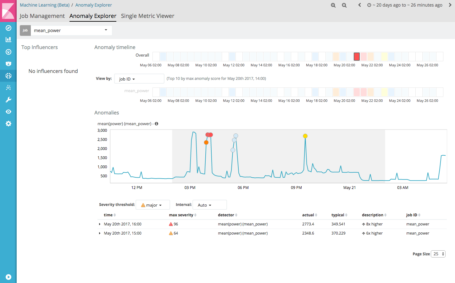
The Anomaly Explorer can be useful if you create multiple, more complex jobs. It will give an overview of the detected anomalies by the different jobs, along with a list of top influencers of the anomalies.

At this point, the mean-power job has been created by feeding it historical data. We can switch to providing the job with a live feed of data, so that it can keep learning and thus improve its performance. To do this, use the following steps:

1. Go to Job Management;
2. Click on the little play button (‘Start datafeed for mean_power’);
3. Select ‘No end time (Realtime search)’;
4. Click the Start button.

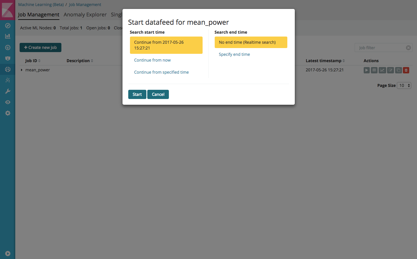
The mean_power job is now ready for future use!

Summary

In this guide we have created a setup with the following components:

• A complete data pre-processing and ingestion pipeline;
• An energy consumption dashboard with visualizations;
• Smart energy consumption insights with anomaly detection.

When indexing time-series data based on single value (energy consumption), these components can be used to:

• Gather insights in our current energy consumption and history;
• Monitor the effect of actions to save energy;
• See trends in energy consumption and project consumption to saving goals;
• Detect anomalies in energy consumption.

Conclusions

Although these capabilities are impressive already, it really starts to get interesting if we scale out a bit to an office building or even a complex of buildings. By feeding multiple sensor data (e.g. temperature, humidity) and climate system or solar panel installation operational data into Elasticsearch, we could monitor the performance of these systems and see if the performance matches the given values of the manufacturer. Furthermore, these insights can be used for a better configuration of these systems, which potentially could lead to a large energy and cost reduction.

After following this guide, one can conclude that X-Pack Machine Learning makes is very easy to add machine learning capabilities to your system. You quickly have a machine learning enabled system up and running, and it is very easy to experiment with. I would love to hear from you if you have any ideas how to integrate X-Pack Machine Learning in your own projects. Also if you have any questions in doing this, please let me know. I am happy to help you out!

About the author

Leon Schrijvers works as a Senior Software Architect at Trifork Eindhoven. He has a passion for data related projects, security and quality control. Leon has a proven track record of designing and implementing online solutions for A-Brands. By doing this, he is the technical conscience of the project and delivers innovative, high quality results. He loves to share knowledgde and share his enthusiasm with others.