Use Kibana to analyze your images

If you are reading some technical blogs, maybe about search or data analysis, chances are big you have read about Kibana. You have seen stories about how easy it is    to use. Most of the blogging effort deals with getting data into kibana using logstash for instance. Maybe some of you have installed Kibana and are using it in combination with logstash. But what if you want to analyze other data. With the most recent release M4, Kibana is better than ever in analyzing other sort of data. In this blog I am going to show you how to create your own dashboard in Kibana. In order to do something useful with Kibana we have to have data. Peter Meijer had a very nice idea to index metadata from all of your images to learn about the type of photo’s that you take. I decided to put this in practice. I used Node.js and the exiftool to obtain metadata from images and store it in elasticsearch.

Goal of the project

Using this project you can scan a directory structure for jpg files. Using the exiftool (see installation instructions later on) you can abstract meta-data from you images and insert them into elasticsearch. Then we want to get information about aperture, focal length, iso, exposure from our photo’s using Kibana.

Installation

You need to install the following libraries. Instructions for installation are on the different websites.

• Exiftool : http://www.sno.phy.queensu.ca/~phil/exiftool/ (tested with version 9.41)
• Elasticsearch : http://www.elasticsearch.org/download (tested with version 0.09.7)
• Kibana : http://www.elasticsearch.org/overview/kibana/installation/ (tested with version 3 Milestone 4)
• Node.js : http://nodejs.org (tested with version 0.10.22)

Setup

First we are going to check if your environment is setup right.

• Elasticsearch : Point your browser to http://localhost:9200, you should see a json object with some information about your cluster.
• Exiftool : This must be available on your path, type exiftool, you should see the man page of exiftool now.
• Node.js : Check if node and npm are on your path, node -v and npm -v should present you the version that you have installed.
• Kibana : Kibana should be pointed to your elasticsearch server. For now I assume you have everything running on your local machine. You can copy all files from kibana to your webserver. I personally like to host it as an elasticsearch plugin. To do this, create a folder kibana/_site in the plugins folder of elasticsearch and copy all the kibana files here. Then point your browser to http://localhost:9200/_plugin/kibana and you should see the interface. Usually with a warning that it cannot find an index.

Now we can obtain the sources and run the program. Clone the github repository. Step into the folder and download the required libraries using npm.

# git clone git@github.com:jettro/nodejs-photo-indexer.git
# cd nodejs-photo-indexer
# npm install

After npm install you should have the folder node_modules with the modules exif2 and walk. The exif2 library is used as an interface to the exiftool library, walk is used to traverse a directory structure. These dependencies are configured in the file package.json. Next step is to initialize the elasticsearch index. We have a node.js command for that. This command deletes the index and recreates the index with the right mapping.

# node initindex

Now you can check the mapping for the created index, browse to the following url (or use curl). This should show you part of the content from the settings.json file. http://localhost:9200/myimages/local/_mapping?pretty

{
  "local" : {
    "_all" : {
      "enabled" : false
    },
    "properties" : {
      "aperture" : {
        "type" : "string"
      },
      "camera" : {
        "type" : "string",
        "index" : "not_analyzed",
        "omit_norms" : true,
        "index_options" : "docs"
      },
      "compensation" : {
        "type" : "string"
      },
      "createDate" : {
        "type" : "date",
        "format" : "yyyy:MM:dd HH:mm:ss"
      },
      "exposure" : {
        "type" : "string",
        "index" : "not_analyzed",
        "omit_norms" : true,
        "index_options" : "docs"
      },
      "focalLength" : {
        "type" : "string",
        "index" : "not_analyzed",
        "omit_norms" : true,
        "index_options" : "docs"
      },
      "iso" : {
        "type" : "integer"
      },
      "lens" : {
        "type" : "string",
        "index" : "not_analyzed",
        "omit_norms" : true,
        "index_options" : "docs"
      },
      "name" : {
        "type" : "string",
        "index" : "not_analyzed",
        "omit_norms" : true,
        "index_options" : "docs"
      },
      "shutter" : {
        "type" : "string",
        "index" : "not_analyzed",
        "omit_norms" : true,
        "index_options" : "docs"
      }
    }
  }
}

As you can see, there are a lot of fields that are not analyzed. This is important since we do not want texts like Canon eos 7d to be analyzed. We want to have it as one term. The same is valid for lens names, exposure and shutter speed. This is it, now is the moment you can start importing images. You can run the app and provide the initial folder to start scanning.

# node app /path/to/your/Pictures

While importing, you should see the log showing which pictures it is indexing and which files it skips. When you have your images in elasticsearch it is time to open kibana in a browser and load the dashboard we have created.

Kibana

We start of with the clean dashboard variant. So in the initial screen choose the Blank Dashboard link. Using this dashboard I can already explain a few of the features.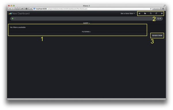

1. Make sure you have the filters toggled on, this way you can see the filters that we later create by clicking on terms.
2. The action buttons from left to right: homescreen, loading saved dashboards, saving the dashboard, sharing the dashboard and configuring the dashboard.
3. Kibana is structured in rows and panels. You can determine the height of the row yourself.

Now we first open the dashboard settings using the gear wheel in the top right of the screen. We can give the dashboard a name, style it, select an index and create and order rows. More settings are available but I do not need those for the demo. Let us give the dashboard a name, add a row and make this row 300px of height. We are going to use this row to show the basic image data: Aperture, exposure and focal length. Than we create a second row to show more information about iso values. We leave the height to 150px. Than we have a third row where we show the camera’s and the lenses. In the final row we add a big table where you can browse all data in a table where you can select the fields you want to show. The following image shows the end result of the configuration of the rows. 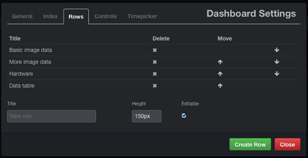Next we are going to add a panel with all the Aperture values that we used for the pictures. This must be added to the first row. Push the button Add panel to empty row. In the popup chose Panel Type terms. Enter the title, field (aperture), length (50), order (term), style (bar) and do not a use a legend. Finally we also do not want to show the amount of images that did not have an aperture. The panel configuration should now look like the following image. And the result looks like the image after that. 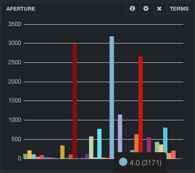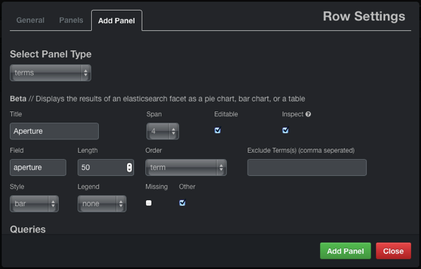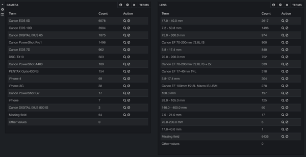The following two panels are similar, we create the bar chart for exposure and focal length. The only difference is the sorting. Now we sort by count, not by term. We move on to the second row. The height is lower than for the first row. Now we are going to create a pie chart for the iOS values. The configuration is almost the same. Some additional presentational options become available. I personally like the Tilt checkbox. As I promised we now are going to present the different camera’s and the lenses I used. I think this is nice to present in a table. So we again select a panel based on terms and than use the table presentation. Again the configuration is not very exciting in configuration. The next images show what we have so far. 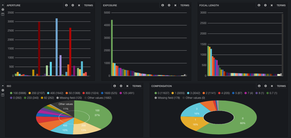Enough information is available to start analyzing our data. Imagine we want to zoom in on all the pictures taken with my Canon EOS 7D. Click on the magnifying glass on the same row as the mentioned camera. Notice that all the graphs change and that we have a Filter now (top of the screen). Notice that in the lenses table I have 7 lenses. Which is not accurate. There is duplication, because all three lenses are twice in the list. Than I still mis one. I also have an extender that I use on the 70-200 lens, this becomes a 140-200 lens. Now let us zoom in on the 70-200 lens. But I want both ways it was written down as well as the ones with the extender. Therefore I omit the other lenses from the result by clicking the hide or delete sign next to the magnifying glass. From the image I can see that when I use my 7D in combination with the 70-200mm lens I most often use aperture 2.8 (which is the maximum of the lens). The exposure is most often 1/250 second and the focal lens is also mostly on the maximum 200 mm. One could argue I need a new lens with more focal length because I am always using the maximum. The next image shows the top part of the screen 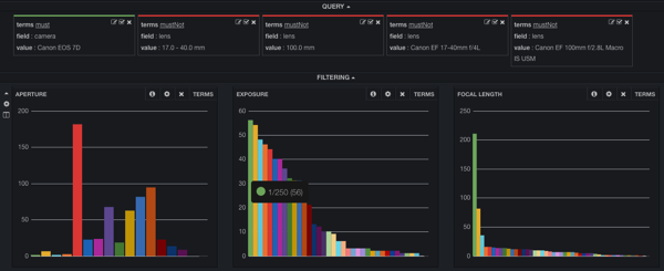We have reached the last part of the demo, row 4. We want to have the overview of all the data where you can select the fields to show. Add a panel to the fourth row of type table. Change the span from 4 to 12. Nothing else needs to be done. Now you get the table with all fields that can be selected. The following image shows this panel.

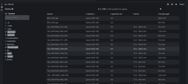
Concluding

I hope this inspires you to start playing with Kibana. I think this is a very nice tool that can be used to do all sorts of data analysis. The only way to learn is to create an index you know and understand and create panels yourself. If you see strange or unexpected results take a good look at the analysis of your data. Elasticsearch comes with great power, but with great power you can make big mistakes. If you want to play around with my index, you can download the index together with the dashboard at this url: http://info.trifork.nl/rs/jteam/images/blog-kibana-example-index.zip  If you want to learn more about logstash and kibana have a look at another blogpost of mine: Oh no, more logs …