An Introduction To Mahout's Logistic Regression SGD Classifier

by frank, February 4, 2014

This blog features classification in Mahout and the underlying concepts. I will explain the basic classification process, training a Logistic Regression model with Stochastic Gradient Descent and a give walkthrough of classifying the Iris flower dataset with Mahout.

Clustering versus Classification

One of my previous blogs focused on text clustering in Mahout. Clustering is an example of unsupervised learning. The clustering algorithm finds groups within the data without being told what to look for upfront. This contrasts with classification, an example of supervised machine learning, which is the process of determining to which class an observation belongs. A common application of classification is spam filtering. With spam filtering we use labeled data to train the classifier: e-mails marked as spam or ham. We then can test the classifier to see whether it has done a good job of detecting spam from e-mail messages it hasn’t seen during the training phase.

The basic classification process

Classification is a deep and broad subject with many different algorithms and optimizations. The basic process however remains the same:

Obtain a dataset
Transform the dataset into a set of records with a field-oriented format containing the features the classifier trains on
Label items in the training set
Split a dataset into test set and training set
Encode the training set and the test set into vectors
Create a model by training the classifier with the training set, with multiple runs and passes if necessary
Test the classifier with the test set
Evaluate the classifier
Improve the classifier and repeat the process

Logistic Regression & Stochastic Gradient Descent

Before we dive into Mahout let’s look at how Logistic Regression and Stochastic Gradient Descent work. This is very short and superficial introduction to this topic but I hope it gives enough of an idea how the algorithms work in order to follow the example later on. I have included links here and there to Wikipedia and videos of the Coursera Machine Learning course for more information.

The Logistic function

Before I discuss Logistic Regression and SGD let’s look it’s foundation, the logistic function. The logistic function is an S-shaped function whose range lies between 0 and 1, which makes it useful to model probabilities. When used in classification, an output close to 1 can indicate that an item belongs to a certain class. See the formula and graph below.

$latex \frac{1}{1+e^{-x}}&s=3$

Logistic function

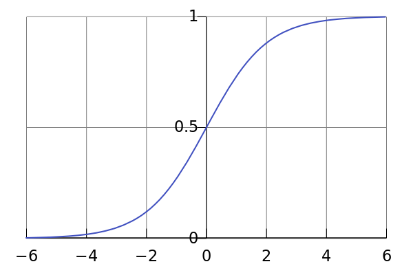
Graph of the logistic function

Logistic Regression model

Logistic Regression builds upon the logistic function. In contrast to the logistic function above which has a single x value as input, a Logistic Regression model allows many input variables: a vector of variables. Additionally, it consists of weights or coefficients for each input variable. The resulting Logistic Regression model looks like this:

$latex \frac{1}{1+e^{-(\beta_0 + \beta_{1} x_{1} + \beta_{2} x_{2} + … + \beta_{n} x_{n})}}&s=3$

Logistic regression model

The goal now is to find the values for $$\beta$$s, the regression coefficients, in such a way that the model can classify data with high accuracy. The classifier is accurate if the difference between observed and actual probabilities is low. This difference is also called the cost. By minimizing the cost function of the Logistic Regression model we can learn the values of the $$\beta$$ coefficients. See the following Coursera video on minimizing the cost function.

Stochastic Gradient Descent

The minimum of the cost function of Logistic Regression cannot be calculated directly, so we try to minimize it via Stochastic Gradient Descent, also known as Online Gradient Descent. In this process we descend along the cost function towards its minimum for each training observation we encounter. As a result, the $$\beta$$ coefficients are updated at every step and eventually as we keep taking steps closer to the minimum the cost is reduced and our model improves.

Classifying the Iris flower dataset

Now that you have a general idea about Logistic Regression and Stochastic Gradient Descent let’s look at an example. The Mahout source comes with a great example to demonstrate the classification process described above. The unit test OnlineLogisticRegressionTest contains a test case for classifying the well-known Iris flower dataset. This is a small dataset from 1936 of 150 flowers with 3 different species: Setosa, Versicolor and Virginica and the width and length of their sepals and petals. The dataset is used as a benchmark for testing classification and clustering algorithms.

The code follows most of the steps of the classification process described above. To follow along make sure you have checked out the Mahout source code. Open OnlineLogisticRegressionTest and look at the iris() test case. In the unit test a classifier is trained which can classify the flowers’ species based on dimensions of the sepals and petals. In the next sections I show how Mahout can be used to train and test the classifier and finally assert its accuracy.

Setup and parsing the dataset

See the code snippet below. The first part of the code concerns with setting up a few data structures and load the test and training sets. We also create two separate Lists, data and target, for the features of the dataset and the classes we want to predict. Note that the type of the target List is Integer because the classes of species will be encoded to Integers via the dictionary based on the order they are processed in the dataset. More on that later. Another List called order is created to shuffle the contents of the dataset.

In the for loop on line 24 we iterate over the lines from the CSV file. In lines 29 to 36 each line is splitted on comma’s into separate fields and all fields put into a vector, which is added to data, the list of vectors. On line 30, the first position of the vector, which corresponds to $$\beta_{0}$$ is set to 1. $$\beta_{0}$$ is also known as the intercept term. Look at the regression graph on the following link to see why we need the intercept. The target variable is the 5th position in the CSV file, hence we use Iterables.get(values, 4) on line 39 to obtain it and add it to target. The other values of the data vector are the remaining variables.

  @Test
  public void iris() throws IOException {

    // Snip ...

    RandomUtils.useTestSeed();
    Splitter onComma = Splitter.on(",");

    // read the data
    List raw = Resources.readLines(Resources.getResource("iris.csv"), Charsets.UTF_8);

    // holds features
    List data = Lists.newArrayList();

    // holds target variable
    List target = Lists.newArrayList();

    // for decoding target values
    Dictionary dict = new Dictionary();

    // for permuting data later
    List order = Lists.newArrayList();

    for (String line : raw.subList(1, raw.size())) {
      // order gets a list of indexes
      order.add(order.size());

      // parse the predictor variables
      Vector v = new DenseVector(5);
      v.set(0, 1);
      int i = 1;
      Iterable values = onComma.split(line);
      for (String value : Iterables.limit(values, 4)) {
        v.set(i++, Double.parseDouble(value));
      }
      data.add(v);

      // and the target
      target.add(dict.intern(Iterables.get(values, 4)));
    }

    // randomize the order ... original data has each species all together
    // note that this randomization is deterministic
    Random random = RandomUtils.getRandom();
    Collections.shuffle(order, random);

    // select training and test data
    List train = order.subList(0, 100);
    List test = order.subList(100, 150);
    logger.warn("Training set = {}", train);
    logger.warn("Test set = {}", test);

Training the Logistic Regression model

Now that all the proper data structures are in place let’s train the Logistic Regression model. The iris test will perform 200 runs. This means that it creates 200 instances of the LR algorithm. Also it will do 30 passes through the training set for each run to improve accuracy of the classifier. Mahout’s Logistic Regression code is based on the pseudocode in the appendix of Bob Carpenter’s paper on Stochastic Gradient Descent.

The LR algorithm is created by instantiating the OnlineLogisticRegression with the number of classes and the number of features. We pass the values 3 and 5 into the constructor of OnlineLogisticRegression because we have 3 classes: Setosa, Versicolor and Virginica and 5 features: the intercept term, the petal length and width, the sepal length and width. The third constructor parameter is used for regularization. See the following Coursera video on regularization.

In the same loop, after 30 passes over the training set we test the classifier. We iterate through the test set and call the classifyFull method which takes a single argument: an observation from the test set. Here it gets interesting: the method returns a Vector with probabilities for each of the classes. This means that the sum of all the elements in it have to add to 1, see the testClassify() method which checks this invariant. To find the class predicted by the classifier we use the method maxValueIndex to find the class with the highest probability.

    // now train many times and collect information on accuracy each time
    int[] correct = new int[test.size() + 1];
    for (int run = 0; run < 200; run++) {       OnlineLogisticRegression lr = new OnlineLogisticRegression(3, 5, new L2(1));       // 30 training passes should converge to > 95% accuracy nearly always but never to 100%
      for (int pass = 0; pass < 30; pass++) {
        Collections.shuffle(train, random);
        for (int k : train) {
          lr.train(target.get(k), data.get(k));
        }
      }

      // check the accuracy on held out data
      int x = 0;
      int[] count = new int[3];
      for (Integer k : test) {
        int r = lr.classifyFull(data.get(k)).maxValueIndex();
        count[r]++;
        x += r == target.get(k) ? 1 : 0;
      }
      correct[x]++;
    }

Assert accuracy

After the we have performed 200 runs, each with 30 passes we will test for accuracy. The snippet below checks whether the List correct does not contain any entries with less than 95% accuracy. Also is checks whether there are no accuracies of 100%, too good to be true, because that would probably indicate a target leak. A target leak is information in the training set that unintentionally provides information about the target class, such as identifiers, timestamps but also very subtle pieces of information.

    // verify we never saw worse than 95% correct,
    for (int i = 0; i < Math.floor(0.95 * test.size()); i++) {
      assertEquals(String.format("%d trials had unacceptable accuracy of only %.0f%%: ", correct[i], 100.0 * i / test.size()), 0, correct[i]);
    }
    // nor perfect
    assertEquals(String.format("%d trials had unrealistic accuracy of 100%%", correct[test.size() - 1]), 0, correct[test.size()]);

Next steps

This blog gave a short overview of Logistic Regression and Stochastic Gradient Descent in Mahout using the Iris dataset as an example. The next step would be to apply the algorithm on a more complex dataset that requires Mahout’s vector encoders. The vector encoders are used to classify text and word like variables instead of using doubles used in the Iris dataset. Other things that are not covered in this blog are ways to evaluate classifiers beyond accuracy. In closing, do you have questions or other feedback? Let me know by leaving a comment!